Machine Learning - (LAB PROGRAMS)

Week 8

☛ Implementation of Logistic Regression using sklearn.

Solution :

Logistic regression:

Logistic regression is one of the most popular Machine Learning algorithms, which comes under the Supervised Learning technique. It is used for predicting the categorical dependent variable using a given set of independent variables. Logistic regression predicts the output of a categorical dependent variable. Therefore the outcome must be a categorical or discrete value. It can be either Yes or No, 0 or 1, true or False, etc. but instead of giving the exact value as 0 and 1, it gives the probabilistic values which lie between 0 and 1.

In this implementation, we use "Study Hours" as the independent variable and "Exam Results (0 or 1)" as the dependent variable.

Steps :

Step 1. Importing Required Libraries

pandas: For loading and processing the dataset.
numpy: For numerical computations, such as generating a range of values for plotting.
matplotlib.pyplot: For creating the graph and visualizing the results.
sklearn.model_selection: For splitting the dataset into training and testing subsets.
sklearn.linear_model: For implementing the logistic regression model.
sklearn.metrics: For evaluating the model’s performance using metrics like accuracy, confusion matrix, and classification report.

Step 2. Reading the Dataset

pd.read_csv() reads the CSV file into a Pandas DataFrame.
The file should contain columns for "Study Hours" and "Exam Result".

Step 3. Defining Features (X) and Target (y)

X stores the independent variable (Study Hours).
y stores the dependent variable (Exam Result).

Step 4. Splitting the Dataset

train_test_split() is used to split the data into training (80%) and testing (20%) sets.
random_state=42 ensures the split is reproducible.

Step 5. Training the Logistic Regression Model

LogisticRegression() initializes the logistic regression model.
model.fit(X_train, y_train) trains the model on the training data.

Step 6. Making Predictions

model.predict(X_test) uses the trained model to predict the exam results for the test set.

Step 7. Evaluating the Model

Accuracy: The percentage of correct predictions, calculated by accuracy_score().
Confusion Matrix: Shows TP, TN, FP, FN for insight into performance.
Classification Report: Provides precision, recall, F1-score, and support for each class.

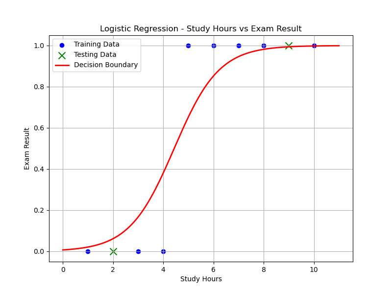
Step 8. Plotting the Data Points and Decision Boundary

Scatter Plot: Displays training data in blue and test data in green (x-shaped).
Decision Boundary: Red line showing model's predicted probabilities for class 1 across study hours.

Library Installation:

To install required libraries, Open Command Prompt or Terminal and execute the following commands


$ pip install scikit-learn

$ pip install numpy

$ pip install pandas

$ pip install matplotlib

CSV file : "study_hours.csv"

Study Hours,Exam Result
1,0
2,0
3,0
4,0
5,1
6,1
7,1
8,1
9,1
10,1

To Download above CSV file : Click Here

Source Code:

File Name: Logistic_Regression.py


import pandas as pd
import numpy as np
import matplotlib.pyplot as plt
from sklearn.linear_model import LogisticRegression
from sklearn.model_selection import train_test_split
from sklearn.metrics import accuracy_score, confusion_matrix, classification_report

# Step 1: Load the dataset
data = pd.read_csv("study_hours.csv")  # Ensure this file exists in the same directory
X = data[['Study Hours']].values
y = data['Exam Result'].values

# Step 2: Train-test split
X_train, X_test, y_train, y_test = train_test_split(
    X, y, test_size=0.2, random_state=42)

# Step 3: Train logistic regression model
model = LogisticRegression()
model.fit(X_train, y_train)

# Step 4: Predict and evaluate
y_pred = model.predict(X_test)

# Step 5: Print results
print(f"Accuracy: {accuracy_score(y_test, y_pred):.1f}")
print("\nConfusion Matrix:")
print(confusion_matrix(y_test, y_pred))

print("\nClassification Report:")
print(classification_report(y_test, y_pred))

# Step 6: Plotting decision boundary
X_range = np.linspace(X.min() - 1, X.max() + 1, 300).reshape(-1, 1)
y_prob = model.predict_proba(X_range)[:, 1]

plt.figure(figsize=(8, 6))
plt.scatter(X_train, y_train, color='blue', label='Training Data')
plt.scatter(X_test, y_test, color='green', marker='x', s=100, label='Testing Data')
plt.plot(X_range, y_prob, color='red', linewidth=2, label='Decision Boundary')
plt.xlabel("Study Hours")
plt.ylabel("Exam Result")
plt.title("Logistic Regression - Study Hours vs Exam Result")
plt.legend()
plt.grid(True)
plt.show()

Output:


Sample Run:
--------------
$ python3 Logistic_Regression.py
Accuracy: 1.0

Confusion Matrix:
[[1 0]
 [0 1]]

Classification Report:
              precision    recall  f1-score   support

           0       1.00      1.00      1.00         1
           1       1.00      1.00      1.00         1

    accuracy                           1.00         2
   macro avg       1.00      1.00      1.00         2
weighted avg       1.00      1.00      1.00         2

Machine Learning Lab Programs

1) Write a python program to compute
• Central Tendency Measures: Mean, Median,Mode
• Measure of Dispersion: Variance, Standard Deviation View Solution

2) Study of Python Basic Libraries such as Statistics, Math, Numpy and Scipy View Solution

3) Study of Python Libraries for ML application such as Pandas and Matplotlib View Solution

4) Write a Python program to implement Simple Linear Regression View Solution

5) Implementation of Multiple Linear Regression for House Price Prediction using sklearn View Solution

6) Implementation of Decision tree using sklearn and its parameter tuning View Solution

7) Implementation of KNN using sklearn View Solution

8) Implementation of Logistic Regression using sklearn View Solution

9) Implementation of K-Means Clustering View Solution

10) Performance analysis of Classification Algorithms on a specific dataset (Mini Project) View Solution

Menu