
Multiple Linear Regression
Solution :
Library Installation:
To install required library files, Open Command Prompt or Terminal and execute the following commands
$ pip install scikit-learn

$ pip install numpy

$ pip install matplotlib
PROGRAM: (Multiple_Linear_Regression.py)
# Import libraries
import numpy as np
import matplotlib.pyplot as plt
from sklearn.linear_model import LinearRegression
from sklearn.model_selection import train_test_split
from sklearn.metrics import mean_squared_error, r2_score

# Sample dataset (2 independent variables)
X=np.array([
    [1, 2],
    [2, 1],
    [3, 4],
    [4, 3],
    [5, 5],
    [6, 7],
    [7, 6],
    [8, 8],
    [9, 9],
    [10, 10]
])

Y=np.array([5, 6, 9, 10, 13, 17, 18, 21, 24, 27])

# Split data
X_train, X_test, Y_train, Y_test=train_test_split(X, Y, test_size=0.2, random_state=42)

# Create model
model=LinearRegression()
model.fit(X_train, Y_train)

# Predict
Y_pred=model.predict(X_test)

# Print coefficients
print(f"Coefficients (slopes): {model.coef_}")
print(f"Intercept: {model.intercept_}")

# Performance metrics
mse=mean_squared_error(Y_test, Y_pred)
r2=r2_score(Y_test, Y_pred)

print(f"Mean Squared Error: {mse}")
print(f"R-squared: {r2}")

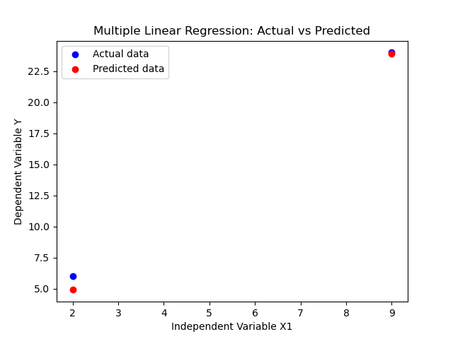
# Visualization (using first feature X1)
plt.scatter(X_test[:, 0], Y_test, color='blue', label='Actual data')
plt.scatter(X_test[:, 0], Y_pred, color='red', label='Predicted data')

plt.title("Multiple Linear Regression: Actual vs Predicted")
plt.xlabel("Independent Variable X1")
plt.ylabel("Dependent Variable Y")
plt.legend()

plt.show()
OUTPUT:
Coefficients (slopes): [1.60343035 0.97089397]
Intercept: 0.7198544698544644
Mean Squared Error: 0.613818475239997
R-squared: 0.9924219941328395
💻 Run This Python Program
Multiple Linear Regression
The selected Python program is loaded
automatically into the editor.
Edit the program, provide input through
STDIN if required
and click Run.
The compiler is embedded using OneCompiler.
Your Python program runs inside the embedded
Python environment; Study Glance does not execute
Python code directly on your web server.
If the program asks for input, type the value in the
STDIN box before clicking Run.
These programs use libraries such as NumPy, Pandas,
Matplotlib, scikit-learn, SciPy and statsmodels, and
graph windows (
plt.show()) cannot be displayed
here. The data files shown in the lesson (CSV) are loaded
into the editor automatically. If a library is not
available in the embedded compiler, use
Copy Program and run the program on your
computer (after pip install of the libraries)
or in Google Colab.