Computational Mathematics [ Lab Programs ]

---

Aim:

☛  
UNIT-IV: First-Order ODEs:
Exact and non-exact equations, Applications: exponential growth/decay, Newton's law of cooling.
Programs:
      • Solving exact and non-exact equations.
      • Solving exponential growth/decay and Newton's law of cooling problems.

Solution :

• Python program for solving exact equations.

PROGRAM: (Exact_Equations.py)

 
import sympy as sp

# Define symbols
x, y = sp.symbols('x y')

# Define M(x,y) and N(x,y)
M = 2*x*y + y**2
N = x**2 + 2*x*y

# Check exactness
dM_dy = sp.diff(M, y)
dN_dx = sp.diff(N, x)

print("dM/dy =", dM_dy)
print("dN/dx =", dN_dx)

if sp.simplify(dM_dy - dN_dx) == 0:
    print("\nEquation is EXACT")

    # Integrate M w.r.t x
    F = sp.integrate(M, x)

    # Differentiate F w.r.t y
    Fy = sp.diff(F, y)

    # Adjust missing terms
    g = sp.integrate(N - Fy, y)

    F = F + g

    print("\nGeneral Solution F(x,y) = C:")
    print(F)

else:
    print("\nNot an exact equation")

OUTPUT:

 
dM/dy = 2*x + 2*y
dN/dx = 2*x + 2*y

Equation is EXACT

General Solution F(x,y) = C:
x**2*y + x*y**2

---

• Python program for solving non-exact equations.

PROGRAM: (Non_Exact_Equations.py)

 
import sympy as sp

# Symbols
x, y = sp.symbols('x y')

# Define M and N (NON-exact example)
M = y
N = -x 

# Step 1: Check exactness
dM_dy = sp.diff(M, y)
dN_dx = sp.diff(N, x)

print("dM/dy =", dM_dy)
print("dN/dx =", dN_dx)

if sp.simplify(dM_dy - dN_dx) == 0:
    print("\nEquation is EXACT")

    # Solve directly
    F = sp.integrate(M, x)
    Fy = sp.diff(F, y)
    g = sp.integrate(N - Fy, y)

    F = F + g

    print("\nSolution F(x,y) = C:")
    print(F)

else:
    print("\nEquation is NON-EXACT")

    # Step 2: Try integrating factor (x-based)
    IF = sp.exp(sp.integrate((dM_dy - dN_dx)/N, x))

    print("\nIntegrating Factor (assumed μ(x)):")
    print(IF)

    # Step 3: Multiply IF with M and N
    M1 = IF * M
    N1 = IF * N

    print("\nAfter applying IF:")
    print("M1 =", M1)
    print("N1 =", N1)

    # Step 4: Now treat as EXACT equation

    print("\nNow solving as EXACT equation...")

    F = sp.integrate(M1, x)
    Fy = sp.diff(F, y)
    g = sp.integrate(N1 - Fy, y)

    F = F + g

    print("\nFinal Solution F(x,y) = C:")
    print(F)

OUTPUT:

 
dM/dy = 1
dN/dx = -1

Equation is NON-EXACT

Integrating Factor (assumed μ(x)):
x**(-2)

After applying IF:
M1 = y/x**2
N1 = -1/x

Now solving as EXACT equation...

Final Solution F(x,y) = C:
-y/x

---

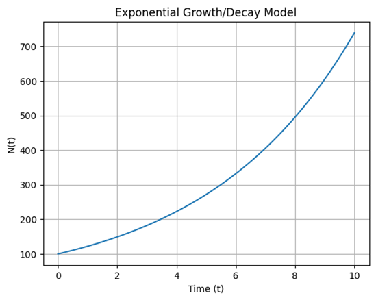
• Python program to find solution for exponential growth/decay.

PROGRAM: (Growth_Decay.py)

 
import numpy as np
import matplotlib.pyplot as plt

# Input values
N0 = float(input("Enter initial value (N0): "))
k = float(input("Enter the exponential growth (positive) or decay (negative) rate k: "))
t_max = int(input("Enter max time: "))

# Time values
t = np.linspace(0, t_max, 100)

# Exponential model
N = N0 * np.exp(k * t)

# Print some values
print("\nTime vs Value:")
for i in range(0, len(t), 20):
    print(f"t={t[i]:.1f}, N={N[i]:.2f}")

# Plot graph
plt.plot(t, N)
plt.xlabel("Time (t)")
plt.ylabel("N(t)")
plt.title("Exponential Growth/Decay Model")
plt.grid()
plt.show()

OUTPUT:

 
Enter initial value (N0): 100
Enter the exponential growth (positive) or decay (negative) rate k: 0.2
Enter max time: 10

Time vs Value:
t=0.0, N=100.00
t=2.0, N=149.79
t=4.0, N=224.36
t=6.1, N=336.06
t=8.1, N=503.37

---

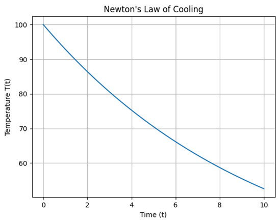
• Python program to find solution for Newton's law of cooling problems.

PROGRAM: (Newtons.py)

 
import numpy as np
import matplotlib.pyplot as plt

# Inputs
T0 = float(input("Enter initial temperature (T0): "))
Ts = float(input("Enter surrounding temperature (Ts): "))
k = float(input("Enter cooling constant (k): "))
t_max = float(input("Enter maximum time: "))

# Time values
t = np.linspace(0, t_max, 100)

# Newton's Law of Cooling formula
T = Ts + (T0 - Ts) * np.exp(-k * t)

# Print sample values
print("\nTime vs Temperature:")
for i in range(0, len(t), 20):
    print(f"t={t[i]:.1f}, T={T[i]:.2f}")

# Plot graph
plt.plot(t, T)
plt.xlabel("Time (t)")
plt.ylabel("Temperature T(t)")
plt.title("Newton's Law of Cooling")
plt.grid()
plt.show()

OUTPUT:

 
Enter initial temperature (T0): 100
Enter surrounding temperature (Ts): 25
Enter cooling constant (k): 0.1
Enter maximum time: 10

Time vs 	Temperature:
t=0.0,	 T=100.00
t=2.0,	 T=86.28
t=4.0, 	T=75.07
t=6.1, 	T=65.91
t=8.1,	 T=58.43
 

---

Related Content :

1.
UNIT - I: Eigen values and Eigenvectors:
Programs:
      • Finding real and complex Eigen values.
      • Finding Eigen vectors.    View Solution

2.
UNIT - II: Solution of Algebraic and Transcendental Equations:
Bisection method, Newton Raphson Method
Programs:
      • Root of a given equation using Bisection method.
      • Root of a given equation Newton Raphson Method.    View Solution

3.
UNIT-III: Linear system of equations:
Jacobi's iteration method and Gauss-Seidal iteration method
Programs:
      • Solution of given system of linear equations using Jacobi's method.
      • Solution of given system of linear equations using Gauss-Seidal method.    View Solution

4.
UNIT-IV: First-Order ODEs:
Exact and non-exact equations, Applications: exponential growth/decay, Newton's law of cooling.
Programs:
      • Solving exact and non-exact equations.
      • Solving exponential growth/decay and Newton's law of cooling problems.    View Solution

5.
UNIT-V: Higher order linear differential equations with constant coefficients:
Programs:
      • Solving homogeneous ODEs.
      • Solving non-homogeneous ODEs.    View Solution