---

Hopfield Networks

---

Hopfield Neural Network

Hopfield neural network was Proposed by John J. Hopfield in 1982. It is an auto-associative fully interconnected single layer feedback network. It is a symmetrically weighted network(i.e., W_ij = W_ji). The Hopfield network is commonly used for auto-association and optimization tasks.

The Hopfield network is of two types

1. Discrete Hopfield Network
2. Continuous Hopfield Network

Discrete Hopfield Network

When this is operated in discrete line fashion it is called as discrete Hopfield network

The network takes two-valued inputs: binary (0, 1) or bipolar (+1, -1); the use of bipolar inpurs makes the analysis easier. The network has symmetrical weights with no self-connections, i.e.,
W_ij = W_ji;     
W_ij = 0    if i = j

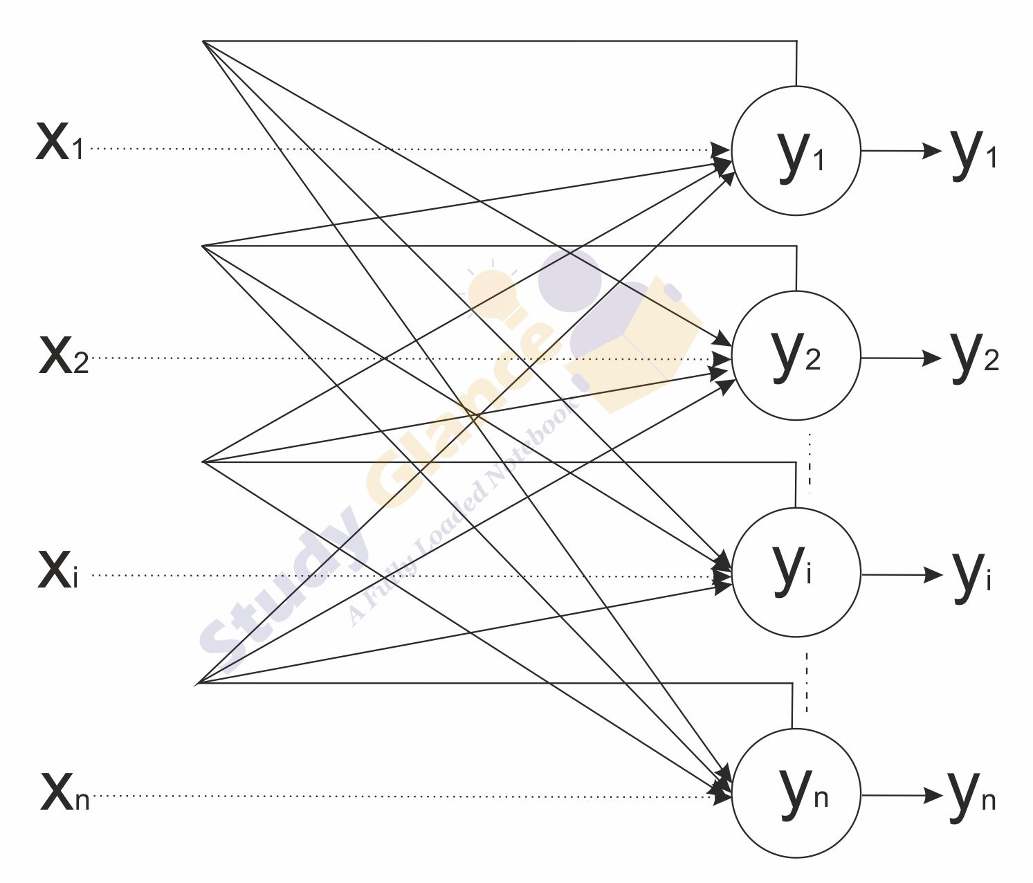
Architecture of Discrete Hopfield Network

The Hopfield's model consists of processing elements with two outputs, one inverting and the other non-inverting. The outputs from each processing element are fed back to the input of other processing elements but not to itself.

Training Algorithm of Discrete Hopfield Network

During training of discrete Hopfield network, weights will be updated. As we know that we can have the binary input vectors as well as bipolar input vectors.

Let the input vectors be denoted by s(p), p = 1, ... , P. Then the weight matrix W to store a set of input vectors, where

In case of input vectors being binary, the weight matrix W = {w_ij} is given by

$$w_{ij}=\underset{p=1}{\overset{P}{\sum <!--\; \sum \; -->}}[2s_i(p)-<!--\; -\; -->1][2s_j(p)-<!--\; -\; -->1]fori\ne <!--\; \ne \; -->j$$

When the input vectors are bipolar, the weight matrix W = {w_ij} can be defined as

$$w_{ij}=\underset{p=1}{\overset{P}{\sum <!--\; \sum \; -->}}[s_i(p)][s_j(p)]fori\ne <!--\; \ne \; -->j$$

---

---

Testing Algorithm of Discrete Hopfield Net

Step 0: Initialize the weights to store patterns, i.e., weights obtained from training algorithm using Hebb rule.

Step 1: When the activations of the net are not converged, then perform Steps 2-8.

Step 2: Perform Steps 3-7 for each input vector X.

Step 3: Make the initial activations of the net equal to the external input vector X: $$y_i=x_{i}fori=1ton$$

Step 4: Perform Steps 5-7 for each unit y_i. (Here, the units are updated in random order.)

Step 5: Calculate the net input of the network: $$y_{ini}=x_i+{\displaystyle \underset{j}{\sum <!--\; \sum \; -->}{y}_j{w}_{ji}}$$

Step 6: Apply the activations over the net input to calculate the output: $$y_i=\{\begin{array}{ll}1& if{y}_{ini}>{\mathrm{\theta <!--\; \theta \; -->}}_i\\ y_i& if{y}_{ini}={\mathrm{\theta <!--\; \theta \; -->}}_i\\ 0& if{y}_{ini}<{\mathrm{\theta <!--\; \theta \; -->}}_i\end{array}$$

where θ_i is the threshold and is normally taken as zero.

Step 7: Now feed back the obtained output y_i to all other units. Thus, the activation vectors are updated.

Step 8: Finally, test the network for convergence.

Continuous Hopfield Network

Continuous network has time as a continuous variable, and can be used for associative memory problems or optimization problems like traveling salesman problem. The nodes of this nerwork have a continuous, graded output rather than a two state binary ourput. Thus, the energy of the network decreases continuously with time.

---

Next Topic :Fixed Weight Competitive Networks