Decision tree induction
Decision Tree
"What is decision tree?" A decision tree is a flowchart-like tree structure, where each internal node (non-leaf node) denotes a test on an attribute, each branch represents an outcome of the test, and each leaf node (or terminal node) holds a class label. The topmost node in a tree is the root node. It represents the best attribute selected for classification.
Decision Tree is a type of data mining technique that is used to build Classification Models. It builds classification models in the form of a tree-like structure, just like its name. This type of mining belongs to supervised class learning.
In supervised learning, the target result is already known. Decision trees can be used for both categorical and numerical data. The categorical data represent gender, marital status, etc. while the numerical data represent age, temperature, etc.
Example:
The following is a typical decision tree. It represents the concept buys_computer, that is, it predicts whether a customer at AllElectronics is likely to purchase a computer. Internal nodes are denoted by rectangles, and leaf nodes are denoted by ovals.
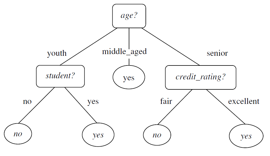
Fig: Decision tree
A decision tree for the concept buys_computer, indicating whether an AllElectronics customer is likely to purchase a computer. Each internal (non-leaf) node represents a test on an attribute. Each leaf node represents a class (either buys_computer = yes or buys_computer = no).
"How are decision trees used for classification?" Given a tuple, X, for which the associated class label is unknown, the attribute values of the tuple are tested against the decision tree. A path is traced from the root to a leaf node, which holds the class prediction for that tuple. Decision trees can easily be converted to classification rules.
Example, According to the decision tree provided above, the tuple (age = senior, credit_rating = excellent) is associated to the class label (buys_computer = yes).
"Why are decision tree classifiers so popular?" The construction of decision tree classifiers does not require any domain knowledge or parameter setting, and therefore is appropriate for exploratory knowledge discovery. Decision trees can handle multidimensional data.
Decision tree induction algorithms have been used for classification in many application areas such as medicine, manufacturing and production, financial analysis, astronomy, and molecular biology.
Decision Tree Induction
In 1980, J. Ross Quinlan, a researcher in machine learning, created the ID3 (Iterative Dichotomiser) algorithm, which is a decision tree algorithm. Later on, he introduced C4.5, which was the successor of ID3. Both ID3 and C4.5 use a greedy approach, where the trees are constructed in a top-down recursive divide-and-conquer manner without any backtracking.
In 1984, a group of statisticians published the book Classification and Regression Trees (CART), which described the generation of binary decision trees. ID3 and CART were invented independently of one another at around the same time, yet follow a similar approach for learning decision trees from training tuples.
Decision Tree algorithm
Generate_decision_tree. Generate a decision tree from the training tuples of data partition, D.
Input:
- Data partition, D, which is a set of training tuples and their associated class labels;
- attribute_list, the set of candidate attributes;
- Attribute_selection_method, describes the method for selecting the best attribute for discrimination among tuples.
Output: A decision tree.
Method:
Step-1: Begin the tree with the root node, say R, which contains the complete dataset D.
Step-2: Find the best attribute in the dataset using Attribute Selection Method (ASM).
Step-3: Divide the R into subsets that contain the possible values of the best attribute.
Step-4: Generate the decision tree node, which contains the best attribute.
Step-5: Recursively make new decision trees using the subsets of the dataset created in step-3. Continue this process until a stage is reached where you cannot further classify the nodes and call the final node a leaf node.
Example: Suppose there is a person who has a job offer and wants to decide whether he should accept or decline the offer. Solve this problem, using the decision tree.
Input:
attribute_list: Salary, Distance and Cab_facility.
class_labels: Accept, Decline.
Method:
- The decision tree starts with the root node (Salary attribute).
- The root node splits further into the next decision node (Distance attribute) and one leaf node based on the corresponding labels.
- The next decision node further gets split into one decision node (Cab_facility attribute) and one leaf node.
- Finally, the decision node (Cab_facility attribute) splits into two leaf nodes (Accept and Decline).
Output:
The below diagram is the decision tree:
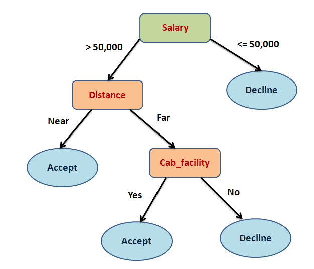
Fig: Decision tree
The algorithm calls Attribute selection method to determine the splitting criterion. The splitting criterion tells us which attribute to test at node N by determining the "best" way to separate or partition the tuples in D into individual classes.
There are three possibilities for partitioning tuples based on the splitting criterion.
Let A be the splitting attribute,
(a) If A is discrete-valued, then one branch is grown for each known value of A.
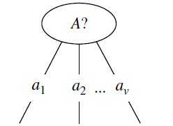
Example:
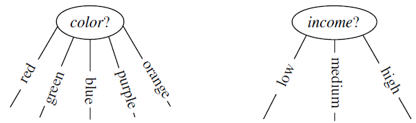
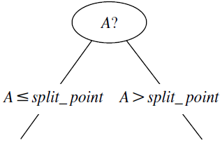
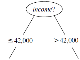
(b) If A is continuous-valued, then two branches are grown, corresponding to A <= split_point and A > split_point.
Example:
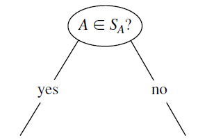
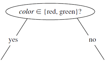
(c) If A is discrete-valued and a binary tree must be produced, then the test is of the form A ∈ SA, where SA is the splitting subset for A.
Example:
Attribute Selection Measures
When implementing a Decision tree, the primary challenge is to choose the most suitable attribute for the root node and sub-nodes. However, there is a technique known as Attribute selection measure that can help resolve such issues. With the help of this measurement, we can easily determine the best attribute for the nodes of the tree.
Here is a list of some attribute selection measures.
- Entropy
- Information gain
Entropy
The calculation of entropy is performed for each attribute after every split, and the splitting process is then continued. A lower entropy indicates a better model, as it implies that the classes are split more effectively due to reduced uncertainty.
It is the measure of impurity (or) uncertainty in the data. For two classes it lies between 0 and 1, and it is calculated using the below formula.
where pi is the nonzero probability that an arbitrary tuple in D belongs to class Ci.
For example, let us see the formula for a use case with 2 classes - Yes and No.
Entropy(D) = −P(Yes)*log2(P(Yes)) − P(No)*log2(P(No))
Here Yes and No are two classes and D is the total number of samples. P(Yes) is the probability of Yes and P(No) is the probability of No.
If there are many classes then the formula is
Entropy(D) = −P1*log2(P1) − P2*log2(P2) − ... − Pn*log2(Pn)
Here n is the number of classes.
Information gain
This method is the main method that is used to build decision trees. It reduces the information that is required to classify the tuples. It reduces the number of tests that are needed to classify the given tuple.
- The attribute with the highest information gain is selected.
- Information gain is basically measuring the change in entropy.
Now, suppose we have to partition the tuples in D on some attribute A having v distinct values, {a1, a2, ..., av}. Then the expected information required to classify the tuple from D based on attribute A is
The term |Dj| / |D| acts as the weight of the jth partition. EntropyA(D) is the expected information required to classify a tuple from D based on the partitioning by A.
Information gain is defined as the difference between the original information requirement and the new requirement (i.e., obtained after partitioning on A)
The attribute A with the highest information gain, Gain(A), is chosen as the splitting attribute at node N.
ID3 Algorithm Example
Let us illustrate the ID3 algorithm with a simple example of classifying whether a customer buys a computer based on some conditions. (or) Construct a decision tree to classify "buys computer."
Consider the following dataset:
| age | income | student | credit_rating | buys_computer |
|---|---|---|---|---|
| youth | high | no | fair | no |
| youth | high | no | excellent | no |
| middle_aged | high | no | fair | yes |
| senior | medium | no | fair | yes |
| senior | low | yes | fair | yes |
| senior | low | yes | excellent | no |
| middle_aged | low | yes | excellent | yes |
| youth | medium | no | fair | no |
| youth | low | yes | fair | yes |
| senior | medium | yes | fair | yes |
| youth | medium | yes | excellent | yes |
| middle_aged | medium | no | excellent | yes |
| middle_aged | high | yes | fair | yes |
| senior | medium | no | excellent | no |
Table-1: customer dataset
Solution
In the given customer dataset, we have 5 attributes/columns, those are age, income, student, credit_rating, and buys_computer.
In which age, income, student, credit_rating attributes are categorized as input features and whereas buys_computer is categorized as output/target feature.
Here, we are going to classify whether a customer buys a computer or not based on the input features. And we will use the ID3 algorithm for building the decision tree.
Let us start the solution:
First, we need to count the number of "yes" and "no" for the output column / feature called "buys_computer." There are 5 "no" and 9 "yes".
So, we will calculate entropy for the output/target variable.
The formula for entropy is
The given dataset has 2 classes - yes and no. Then the formula of Entropy for buys_computer is
Entropy(buys_computer) = −P(yes)*log2(P(yes)) − P(no)*log2(P(no))
Where,
- P(yes) = p(yes) / (p(yes) + p(no)) = 9 / (9 + 5) = 9/14 for the "yes" component of buys_computer.
- P(no) = p(no) / (p(yes) + p(no)) = 5 / (9 + 5) = 5/14 for the "no" component of buys_computer.
Let us substitute the values in the entropy formula,
Entropy(buys_computer) = − (9/14) *log2(9/14) − (5/14) *log2(5/14)
= − (0.64) *log2(0.64) − (0.36) *log2(0.36)
= 0.412 + 0.53
= 0.94 bits
Once we are ready with the Entropy of the target variable, we will find out the Entropy for each column/variable/attribute with respect to the target variable to find the most homogeneous sample.
Let's extract the age column from the given dataset.
| age | buys_computer | Total | |
|---|---|---|---|
| yes | no | ||
| youth | 2 | 3 | 5 |
| middle_aged | 4 | 0 | 4 |
| senior | 3 | 2 | 5 |
| Total | 9 | 5 | 14 |
So, here we can see that
- youth has 2 yes, 3 no
- middle_aged has 4 yes and 0 no
- senior has 3 yes and 2 no.
Now we can calculate the Entropy for each value of age column.
Entropy(youth) = − (2/5) *log2(2/5) − (3/5) *log2(3/5) = 0.97
Entropy(senior) = − (3/5) *log2(3/5) − (2/5) *log2(2/5) = 0.97
Entropy(middle_aged) = − (4/4) *log2(4/4) − (0/4) *log2(0/4) = 0.0
The Entropy of middle_aged is 0 i.e., middle_aged has only the "yes" component.
Note: If the Entropy is Zero (0), that subset is called a pure subset.
So, once we are ready with the Entropy for each value in the age column, we will find out the Entropy for the complete age column with respect to the buys_computer column.
Entropy (buys_computer, age) = P(youth) * E(youth) + P(middle_aged) * E(middle_aged) + P(senior) * E(senior)
= (5/14) * 0.97 + (4/14) * 0 + (5/14) * 0.97
= 0.693 bits
Now, we need to calculate the information gain of column age:
Information Gain (buys_computer, age) = Entropy(buys_computer) − Entropy (buys_computer, age)
= 0.94 − 0.693
= 0.247 bits
Similarly, we can compute Information Gain (buys_computer, income) is 0.029 bits, Information Gain (buys_computer, student) is 0.151 bits, and Information Gain (buys_computer, credit_rating) is 0.048 bits.
The attribute age has the highest information gain and therefore becomes the splitting attribute at the root node of the decision tree. Branches are grown for each outcome of age. The tuples are shown partitioned accordingly.
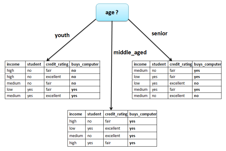
Notice that the tuples falling into the partition for age = middle_aged all belong to the same class. Because they all belong to class "yes," a leaf should therefore be created at the end of this branch and labelled "yes."
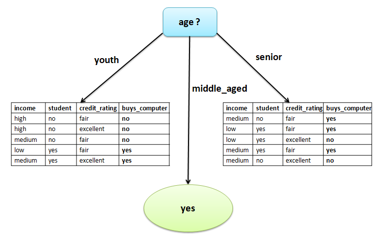
Fig: Decision tree for age attribute.
Let's continue with the next level. If the age is "youth" then the dataset is
| income | student | credit_rating | buys_computer |
|---|---|---|---|
| high | no | fair | no |
| high | no | excellent | no |
| medium | no | fair | no |
| low | yes | fair | yes |
| medium | yes | excellent | yes |
In the above, income, student and credit_rating are categorized as input attributes and buys_computer is categorized as the output attribute. There are 5 instances, among those 2 yes and 3 no for the buys_computer attribute.
Now, we will calculate the Information Gain for all the attributes with respect to the target/class attribute called buys_computer. To calculate Information Gain first, we need to calculate the Entropy for all the attributes.
Let's calculate the Entropy for the class/target attribute buys_computer:
Entropy (buys_computer) = −P(yes)*log2(P(yes)) − P(no)*log2(P(no))
= − (2/5) *log2(2/5) − (3/5) *log2(3/5)
= 0.97 bits
Once we are ready with the Entropy of the target variable, we will find out the Entropy for each column/variable/attribute with respect to the target variable to find the most homogeneous sample.
Let's extract the income attribute from the given dataset.
| income | buys_computer | Total | |
|---|---|---|---|
| yes | no | ||
| low | 1 | 0 | 1 |
| medium | 1 | 1 | 2 |
| high | 0 | 2 | 2 |
| Total | 2 | 3 | 5 |
So, here we can see that
- low has 1 yes, 0 no
- medium has 1 yes and 1 no
- high has 0 yes and 2 no.
Now we can calculate the Entropy for each value of the income column.
Entropy (low) = − (1/1) *log2(1/1) − (0/1) *log2(0/1) = 0
Entropy (medium) = − (1/2) *log2(1/2) − (1/2) *log2(1/2) = 1
Entropy (high) = − (0/2) *log2(0/2) − (2/2) *log2(2/2) = 0
So, once we are ready with the Entropy for each value in the income column, we will find out the Entropy for the complete income column with respect to the buys_computer column.
Entropy (buys_computer, income) = P(low) * E(low) + P(medium) * E(medium) + P(high) * E(high)
= (1/5) * 0 + (2/5) * 1 + (1/5) * 0
= 0.4 bits
Now, we need to calculate the information gain of the column income:
Information Gain (buys_computer, income) = Entropy (buys_computer) − Entropy (buys_computer, income)
= 0.97 − 0.4
= 0.57 bits
Similarly, we can compute Information Gain (buys_computer, student) and Information Gain (buys_computer, credit_rating).
Information Gain (buys_computer, student) = Entropy (buys_computer) − Entropy (buys_computer, student)
= 0.97 − 0
= 0.97 bits
Information Gain (buys_computer, credit_rating) = Entropy (buys_computer) − Entropy (buys_computer, credit_rating)
= 0.97 − 0.951
= 0.020 bits
The attribute student has the highest information gain and therefore becomes the splitting attribute at the next level node of the decision tree. Branches are grown for each outcome of student. The tuples are shown partitioned accordingly.
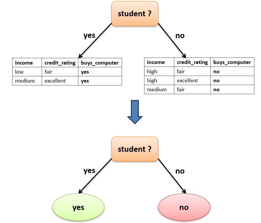
Fig: Decision tree for student attribute.
Notice that the tuples falling into the partition for student = yes all belong to the same class. Because they all belong to class "yes," a leaf should therefore be created at the end of this branch and labelled "yes." The partition for student = no also belongs to a single class, so a leaf should be created at the end of this branch and labelled "no."
Let's continue the same process for the age is "senior".
If you continue the above process then we will get the attribute credit_rating has the highest information gain and therefore becomes the splitting attribute at the next level node of the decision tree. Branches are grown for each outcome of credit_rating. The tuples are shown partitioned accordingly.
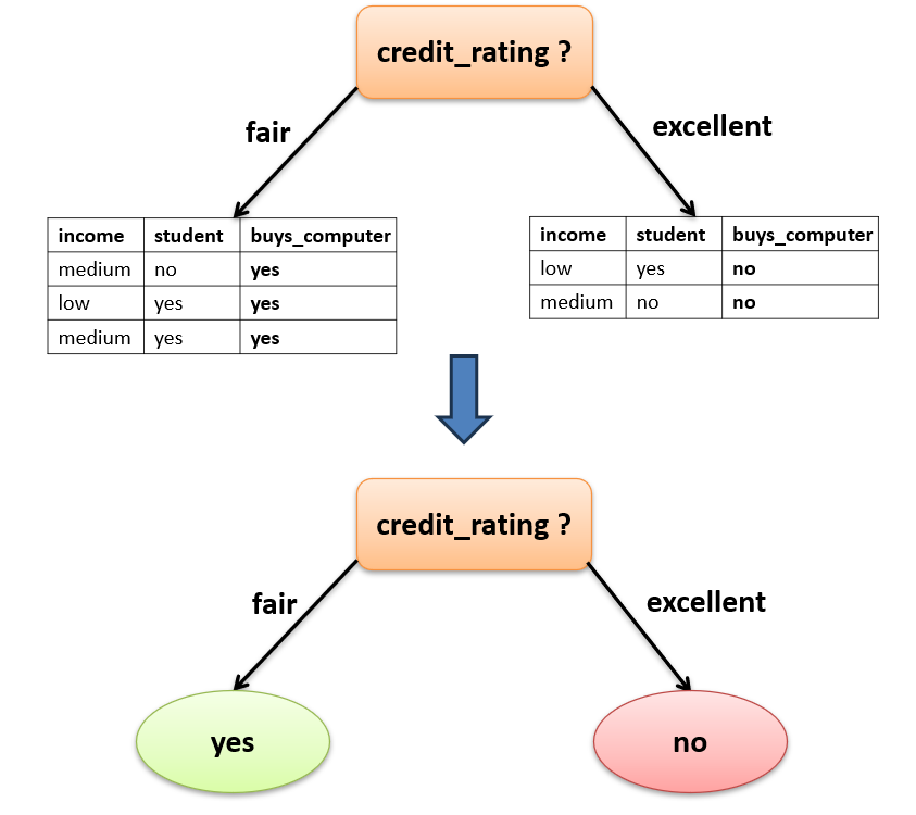
Fig: Decision tree for credit_rating attribute.
Now, we will reach the leaf nodes of the decision tree. i.e., we have derived class labels for all the branches of the dataset.
The final decision tree for the above dataset using the ID3 algorithm:
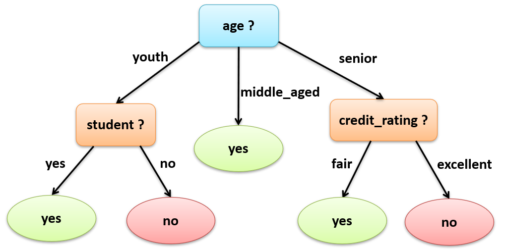
Fig: Decision tree
Exercise: ID3 Algorithm
Let us illustrate the ID3 algorithm with a simple example of classifying golf play based on weather conditions. (or) Construct a decision tree to classify "golf play."
Consider the following dataset:
| Outlook | Temperature | Humidity | Wind | Golf_Play |
|---|---|---|---|---|
| Sunny | Hot | High | Weak | No |
| Sunny | Hot | High | Strong | No |
| Overcast | Hot | High | Weak | Yes |
| Rain | Mild | High | Weak | Yes |
| Rain | Cool | Normal | Weak | Yes |
| Rain | Cool | Normal | Strong | No |
| Overcast | Cool | Normal | Strong | Yes |
| Sunny | Mild | High | Weak | No |
| Sunny | Cool | Normal | Weak | Yes |
| Rain | Mild | Normal | Weak | Yes |
| Sunny | Mild | Normal | Strong | Yes |
| Overcast | Mild | High | Strong | Yes |
| Overcast | Hot | Normal | Weak | Yes |
| Rain | Mild | High | Strong | No |